


Hi everyone 🤗
One of the things I've always wanted to do is to release a robust and reliable prediction model for football matches, and I think I finally achieved something worth sharing.
This post is structured into two sections.
- The end-of-the-season projections for each side in the Premier League.
- The basic assumptions behind the model, for those interested.
Before each Matchday, I'll update my end-of-the-season projections and post detailed naive and biased forecasts (more on this later) for each fixture. Furthermore, I'll assess the model's performance and compare it against FiveThirtyEight's predictions – so, I'm really hoping we beat them 💪.
If you're interested in receiving these posts straight to your inbox and not missing an update, make sure you're subscribed to the newsletter; you can expect the Matchday 1 numbers between Wednesday and Thursday.
Let's get to it!
End-of-the-season Predictions
The following table showcases the probability my model is assigning each team of winning the title, qualifying for a Champions League spot (UECL), and being relegated. Plus, it also showcases the projected final point tally for each side.
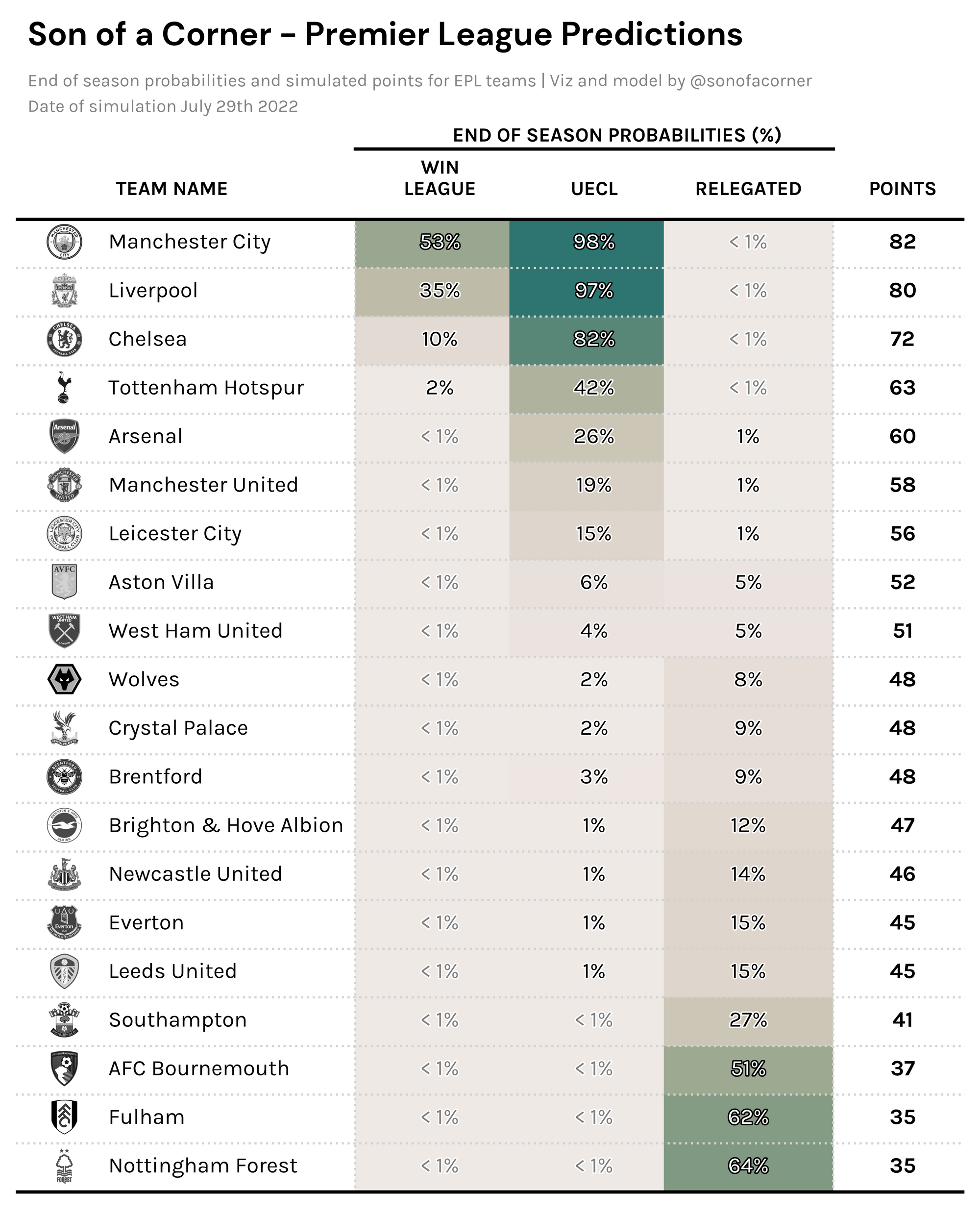
No major surprises here, City and Liverpool are favorites to win the title and the remaining top 4 spots are most likely to be contested between Chelsea, Spurs, and Arsenal.
What did surprise me though, was that aside from the newly promoted sides, Southampton is considered the most likely to be relegated – even ahead of Leeds United who I would've imagined would be in more danger. I also think that it might be underestimating Brighton, and may be too optimistic about Leicester's season.
How do my projections compare to FiveThirtyEight's model?
The following table shows the relative difference between the points projected by my model and FiveThirtyEight's – a positive percentage means I've projected a better outcome for that team, and vice-versa.
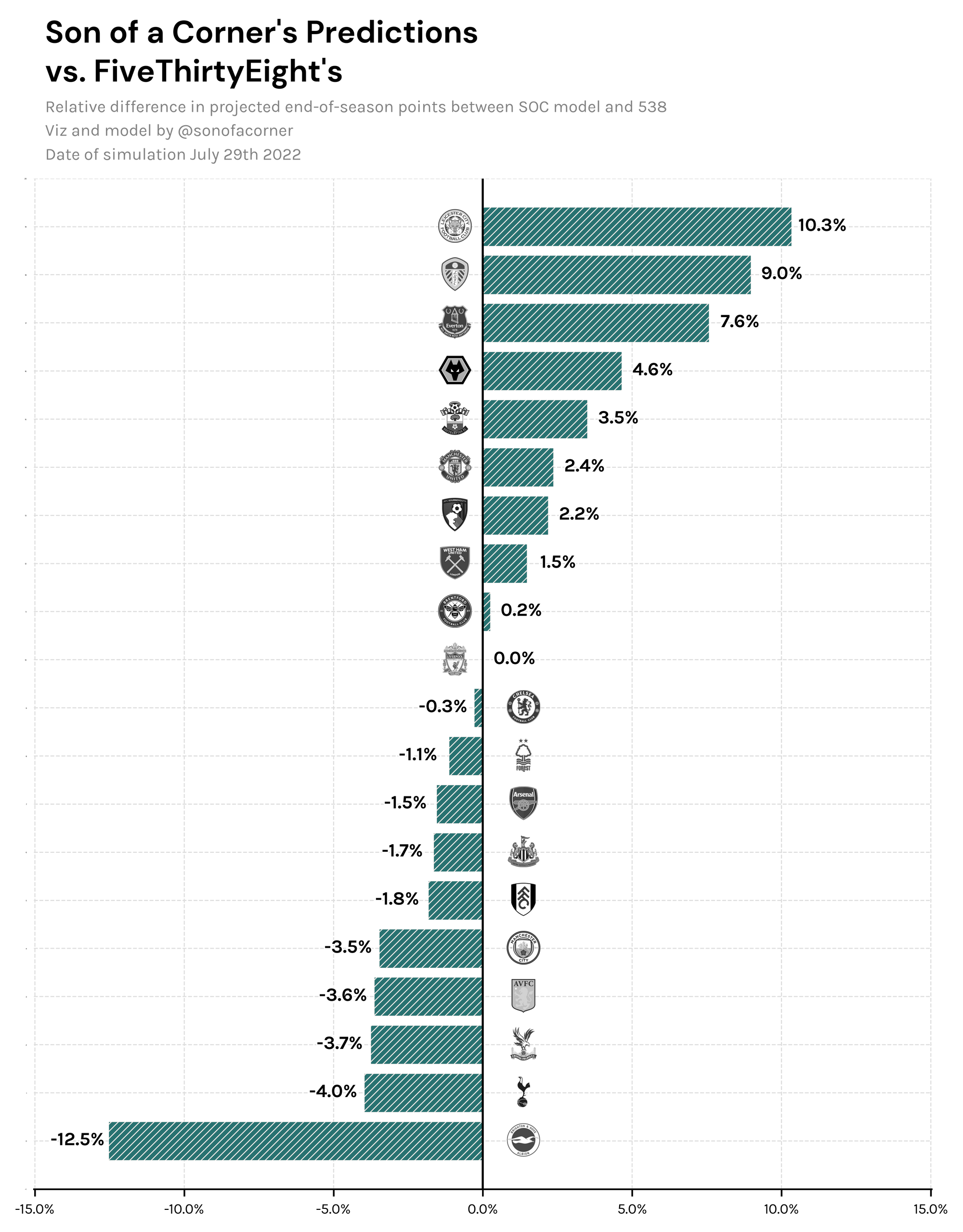
These results give me confidence that my model is on the right track, and barring Brighton's and Leicester's projections I can fairly say that both models are quite aligned with each other.
My main guess on why Brighton are so low on my model is because I don't use expected goals for my projections – which FiveThirtyEight do – and this is a team that has historically underperformed their xG metrics.
How does it work?
The model is structured around three main components, that when piled together, make a great forecast system (at least, I think so).
In this section, I won't get at all into the maths or anything too technical, as I'd rather explain what makes this model different.
Modeling a football match with the Poisson distribution
Most statisticians agree that the best way to model a football match is by using a Poisson distribution, which essentially models the number of occurrences of an event within a certain timeframe.
To achieve this, the Poisson distribution receives a fixed parameter, usually called lambda, which specifies the rate of occurrence of these events. If the lambda is known, then the distribution gives us the probability of the event occurring X times.
In the case of a football match, the events are the goals to be scored by each team and the lambda is the scoring rate of each team. Since we can't really know the actual scoring rate of a team for a particular match, we then have to do some inference on historical data and estimate the parameter. There are many ways to do this. One could be performing a regression on the data, or another option could be something as simple as computing the team's historical average scoring rate.
For this model, I use a Poisson distribution to model each match, but I do it under a Bayesian framework which is a very powerful mathematical theory in the field of statistics.
Bayesian framework
The main difference between the Bayesian framework and classical methods is that it doesn't treat frequency and probability as equivalent. This basically means, in very simplistic terms, that just because Man City have won four of the last five titles, it doesn't mean that there's an 80% chance that they'll win it again this year – at least that's what a Bayesian statistician would say in the matter.
This difference is significant when treating a problem with uncertainty, so let's look at an example.
Imagine that we estimate Brighton's scoring rate (the lambda) to be 1.3 goals per game, and then use this rate to model the goals for a particular match with the Poisson distribution. With a classical framework, our model would not make any distinction between this estimated parameter and a true parameter, despite the former being uncertain. Here's where Bayesian statistics come in handy, as they consider the uncertainty associated with our projected goal rate and reflect it in the output.
An even more incredible thing about a Bayesian framework is that, by nature, it allows us to incorporate prior knowledge into our forecasts. That is, it lets us bias our forecast (or model) without committing any mathematical crimes or inconsistencies. This comes in handy because the person performing the prediction may know something about the problem without it being necessarily apparent in the data.
A great example of this is when it comes to modeling a football match. Yes, Liverpool might have a great historical record. Still, what if, just before the game, most key players become ruled out because of COVID – no model would be able to incorporate this, so we bias our model using our prior knowledge. You can also bias the model without any particular reason whatsoever and just do so because you have a "hunch".
How this prior knowledge is incorporated varies depending on the model, but you can get some idea here.
💡 Prior knowledge must be fed to the model before looking at the data, that's why it's called "prior".
📝 For matchdays, I'll post two forecasts, a naive forecast which doesn't incorporate prior knowledge and a biased forecast with my own hunches for each game.
Clustering and sampling
No matter who you support, I think we can all agree that it's not the same thing for a team to face Liverpool at Anfield and to play Southampton at home.
This is why it's important that we're careful when we select the data to be used as the sample for each match. For this model, I cluster teams into groups based on their transfermarkt valuation and SPI rating at each point in time, and assign the cluster a label that is consistent across time.
Here's an old example of how this works, but please note that it's not the exact clustering that I used for the current model
1/ New viz 📈
— Son of a corner (@sonofacorner) June 2, 2022
I used transfermarkt data and 538's SPI to partition EPL sides into clusters using kmeans.
Here's what I got 👇
Honestly, a bit disappointed that United creeped in with the big guys because of their big fat wallets 💸
(And yes, I did standardize the data) pic.twitter.com/4fsb6j0bdj
Then I use these buckets to sample the historical data. The best way to explain this is with an example, so let's imagine we're modeling the match between Crystal Palace and Arsenal.
Let's say that at the time of the match, my clustering algorithm classified Arsenal in bucket number two, and Palace in bucket number four. My code then takes all the previous matches (all the way back to the 2016 season) in which Arsenal played a team in bucket number two, and in which Arsenal was in bucket number four – plus, taking into account only matches in which Arsenal played away from home, and vice-versa – which is done to consider home advantage.
This is extremely helpful to filter out the noise of games in which Arsenal faced a more difficult opponent and to only consider similar games in the sample. Plus, there are rare occasions when this benefits certain mid-table teams that might overperform against the "big-boys" or vice-versa.
For promoted teams, it gets a bit trickier, but essentially, what the model does is that it considers all promoted teams as "equal" – considering that they belong to the same cluster or bucket. The clustering part helps in differentiating certain promoted sides, which might be different from each other. For example, Forest are in a different bucket than Fulham and Bournemouth, according to my algorithm.
Finally, to account for recent form, my code takes the previous five matches that each side played against teams in a neighboring cluster of their opponent and adds them to the sample (if they weren't contained in the initial filter). This means that, if we go back to our original example of the Palace versus Arsenal fixture, we would add the last five matches in which Palace played a team in a bucket close to Arsenal's. The objective of this is to filter out noise that might come from a difficult set of fixtures, so we don't punish or benefit teams unfairly simply because of their schedule.
Convinced?
As for pitching my model, that's all I got.
I would've liked to add the results of the model's performance tests, but I just didn't have the time to get the visuals in a nice format and I'll update the post at some time during the weekend (I hope).
I really hope you enjoy following these predictions and that the model explanation has helped you in motivating you to learn more about Bayesian statistics.
If you have any questions please reach out on Twitter or email me at theson@sonofacorner.com.
Catch you Monday with the Viz of the Week 👋


