


Hi everyone!
Welcome to a new SOC tutorial. In these series of tutorials (or lessons) we'll explore the basic concepts required to build a simple Bayesian model that estimates the probability that a team will either win, draw or lose a particular fixture.
This first post presents the mathematical concepts used to build the model behind my Premier League forecasts. In this post, we won't go into any code. However, it should provide you with the basic elements to understand the ideas behind Bayesian statistics and how they can be applied to building a model that forecasts the outcome of football matches.
Let's get started.
The Mathematics
For this post, we'll be focused on introducing a couple of mathematical concepts and formulas so that the foundations of our model are well-cemented.
The Poisson Distribution
When it comes to modeling football results, it is usually assumed that the number of goals scored within a match follows a Poisson distribution, where the goals scored by team A are independent of the goals scored by team B.
Essentially, a Poisson distribution is a discrete probability distribution that returns the probability of observing a certain number of occurrences within a fixed interval of time, i.e., the number of goals scored in the space of ninety minutes (in our case).
The Poisson distribution follows a simple formula, where if we let \(X\) be the random variable that represents the number of goals scored by a certain team within a match, we have that: \[ \mathrm{Pr}(X = x) = \frac{\lambda^x e^{-\lambda}}{x!} \]
where \(\lambda > 0\) is a parameter that represents the scoring rate of the team and \(e\) is a constant (Euler's number).
Let's say, for example, that we have that a team's scoring rate \(\lambda = 1.3\). Then, according to the formula above, we would have that the probability of the team scoring \(3\) goals in the match equals: \[ \mathrm{Pr}(X = 3 | \lambda =1.3) = \frac{1.3^3e^{-1.3}}{3!} \approx 0.09979 \]
Simple, right?
To illustrate the idea, we can take each team's observed goal rate \((\lambda)\) and use it as an input for the Poisson distribution to compare it with the distribution of actual goals scored during a single season.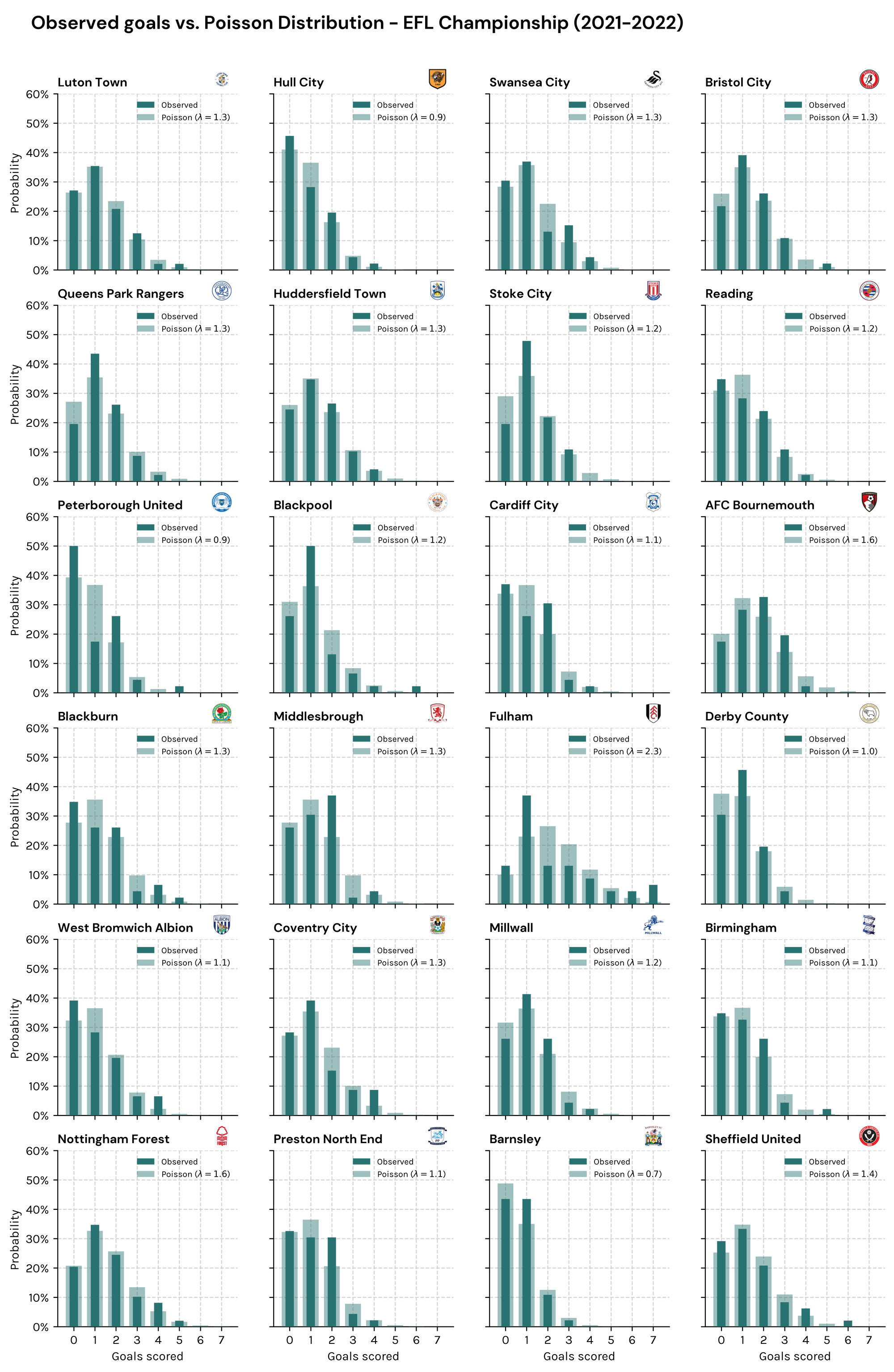
As you can see, the probabilities obtained from the Poisson distribution compare fairly well to the actual goal-scoring distribution for most of the teams in the English Championship.
The Uncertainty of Lambda
Ok, now that we've established that the Poisson distribution could be an appropriate choice for the base of our model, it's time to get into the details of going Bayesian.
Son of a Corner has a membership program, through which members can support the creation of all of the public content published in the site. One of the few ways to say thank you to paid members is by providing them with early access to tutorials. 🤗
If you wish to learn more on how to support Son of a Corner financially, you can do so here.
As mentioned before, the Poisson distribution relies on a single parameter (lambda). However, the main issue with lambda is that it is uncertain. That is, we can't know a team's actual scoring rate going into a match, as it depends on various factors, such as injuries, fatigue, playing style, quality of the opposition, etcetera.
Therefore, our best way forward is to try and estimate the value of lambda by collecting relevant data that helps us come up with a value that best reflects the team's scoring rate based on previous performances.
The key difference in taking a Bayesian approach, as opposed to a frequentist (or classical) statistical approach, is how we perceive the uncertainty behind our knowledge of lambda.
In a frequentist perspective, probability is conceived as the long-run frequency of events, which essentially means that if we have seen an event occur 50% of the time across a big enough time frame, then the probability that we will observe it again equals 50%.
However, in a Bayesian framework, probability is centered around the concept of beliefs or confidence that the event will occur. This is a powerful idea, as it allows for conflicting beliefs based on an individual or personal level. Note that this doesn't disregard any of the rigor behind probability theory since the way we assign those beliefs must always be consistent with the axioms of probability theory.
To put this into the context of our problem, this means that if we took a frequentist approach, we would estimate the value of lambda (via regression, a simple average, or another method) and then take that output and input into our model to compute the probabilities that the team will score x goals in the match.
In a Bayesian framework, things will be quite different, as we will preserve the uncertainty behind our knowledge of lambda and incorporate it into our model.
How can we do that?
By assuming that lambda is a random variable that follows a particular probability distribution. This distribution which is solely dependent on our uncertainty behind the true nature of lambda is usually called the prior distribution of our parameter.
Prior Distributions
As we previously stated, our model assumes that the number of goals scored in any football match follows a Poisson distribution. That is, if we let \(X\) be the number of goals scored by a certain team within a match, then \[ \begin{align} X &\sim \mathrm{Poisson}(\lambda),\\ \mathrm{Pr}(X = x) &= \frac{\lambda^xe^{-\lambda}}{x!} \end{align} \]
Since the main objective of our analysis is to predict a future observation of the unknown value \(X^*\) and where we have an unknown rate parameter \(\lambda\), we can then make use of the Law of total probability to arrive at a predictive distribution for \(X^*\), that is \[ \mathrm{Pr}(X^*) = \int_0^\infty\mathrm{Pr}(X^* | \lambda)\mathrm{Pr}(\lambda)d\lambda. \]
Where \(\mathrm{Pr}(X^* | \lambda) \times \mathrm{Pr}(\lambda)\) is simply the probability of observing \(x^*\) given \(\lambda\), weighed by the probability that \(\lambda\) is the team's actual goal rate.
Now, here's where it gets interesting, as we can simply choose how we wish \(\lambda\) to be distributed based on our beliefs of the true nature of \(\lambda\). Our choice for this distribution is what is called the prior distribution of our parameter.
For the particular case of the Poisson distribution, the most appropriate choice for our prior is for lambda to follow a Gamma distribution – as it provides certain mathematical properties that will make our work easier (for more info on this, check the Wikipedia article on conjugate priors). Essentially, it will turn our previous formula into the following.
\[ \begin{align*} \mathrm{Pr}(X^*) &= \int_0^\infty\mathrm{Pr}(X^* | \lambda)\mathrm{Pr}(\lambda)d\lambda,\\ &= \int_0^\infty\frac{\lambda^{x^*}e^{-\lambda}}{x^*!}\times\frac{\beta^\alpha}{\Gamma(\alpha)}\lambda^{\alpha - 1}e^{-\beta\lambda}d\lambda,\\ &= \frac{\Gamma(x^* + \alpha)}{\Gamma(\alpha)\Gamma(x^* + 1)}p^{\alpha}(1-p)^{x^*}, \end{align*} \]
where \(\alpha, \beta > 0\) are the parameters of the Gamma distribution and \(p = \beta(\beta+1)^{-1}\).
If you're familiar with some probability distributions, you'll notice that \(X^*\) now follows what is called a Poisson Gamma distribution or a Negative Binomial distribution (in the case that \(\alpha\) and \(\beta\) are integers).
The key thing here is that since we now assume that lambda is a random variable, all of our predictions of the number of goals will become a weighted average of a Poisson distribution with all possible lambda values.
This is a huge improvement for the model since we are now factoring all of this uncertainty behind the team's goal rate into our model.
Now, how can we use this to make predictions?
We choose the prior values for our parameters (\(\alpha\) and \(\beta\)) and input them into our formula. Since a Gamma distribution has a mean of \(\frac{\alpha}{\beta}\) and variance of \(\frac{\alpha}{\beta^2}\), we can intuitively choose these parameters to model our beliefs on the team's goal rate. That is, \(\beta\) will play the role of an artificial sample size of matches played, and \(\alpha\) will represent the total number of goals scored during those matches.
A Simple Example
Let's suppose that we have a hypothetical football match where we wish to estimate the number of goals that Bayesian Wanderers will score against Frequentist Albion.
Since our hunch tells us that Bayesian Wanderers have powerful attacking players that could exploit the Frequentist's frail defense, we can tell our model that we believe that the Bayesians would have an average goal rate of 2.3 goals per match against their opponents.
Therefore, our prior parameters \(\alpha\) and \(\beta\) would have to satisfy the following equality \[\frac{\alpha}{\beta} = 2.3,\] where \(\alpha\) will be represent artifical goal sample and \(\beta\) the artificial sample size.
As you might expect, the higher the \(\beta\) (or "sample size") the higher the confidence in our prior beliefs and the less variance present in the probability distribution of \(\lambda\) (the team's goal rate). To illustrate the idea here's a simple visual showcasing different combinations for \(\alpha\) and \(\beta\) that satisfy our previous equation.
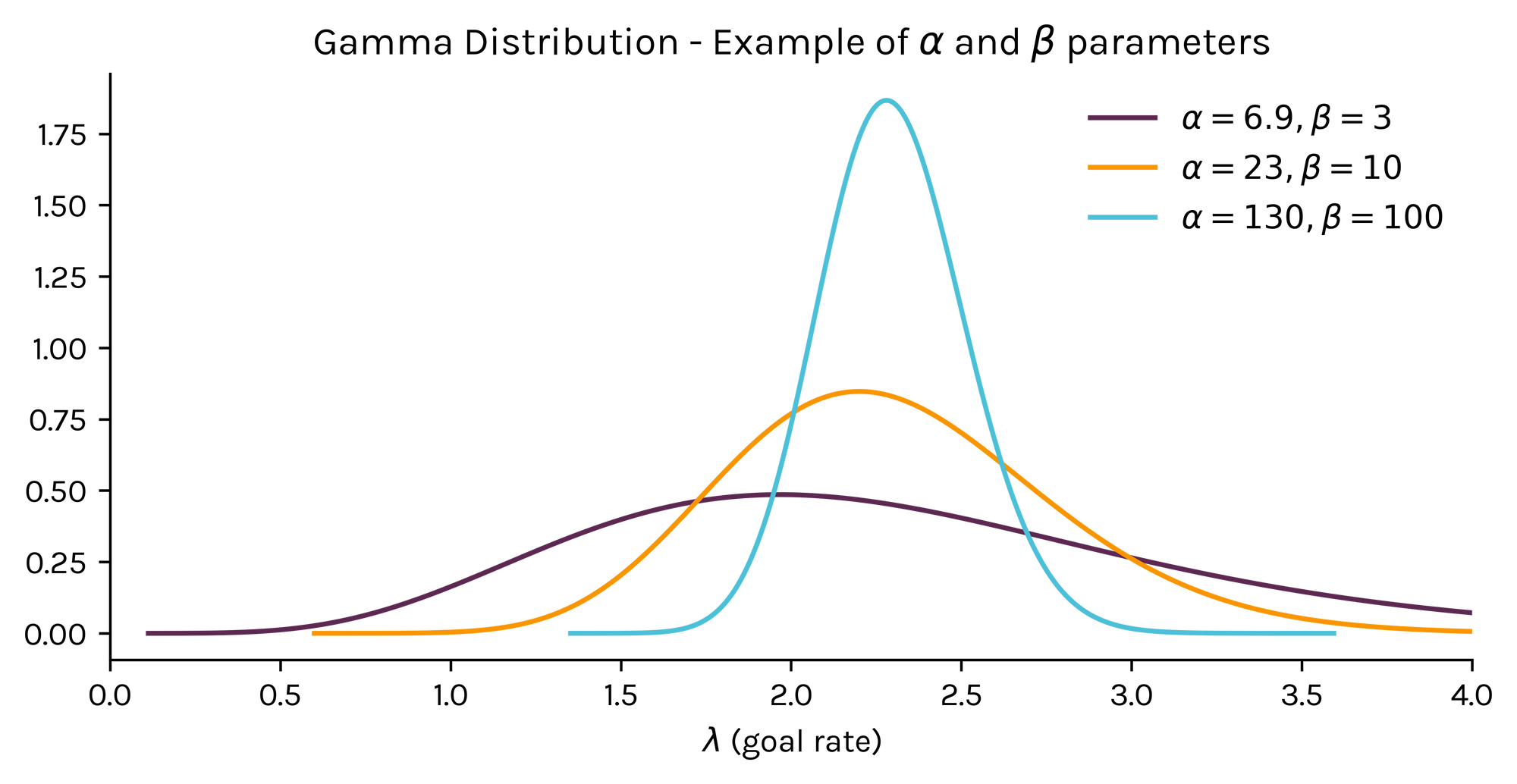
Notice the massive differences in the distributions, despite all of them having an expected value (or mean) of 2.3.
As you can see, the purple line – which assumes an artificial sample size of 3 matches – shows that there is a significant chance for lambda to take multiple values. Whereas, the light blue line (with a prior beta of a 100 matches) is narrowly centered around 2.3.
Now, let's take it one step further and plot the Poisson Gamma distribution that derives from these priors to get the estimated probability that Bayesian Wanderers will score x amount of goals.
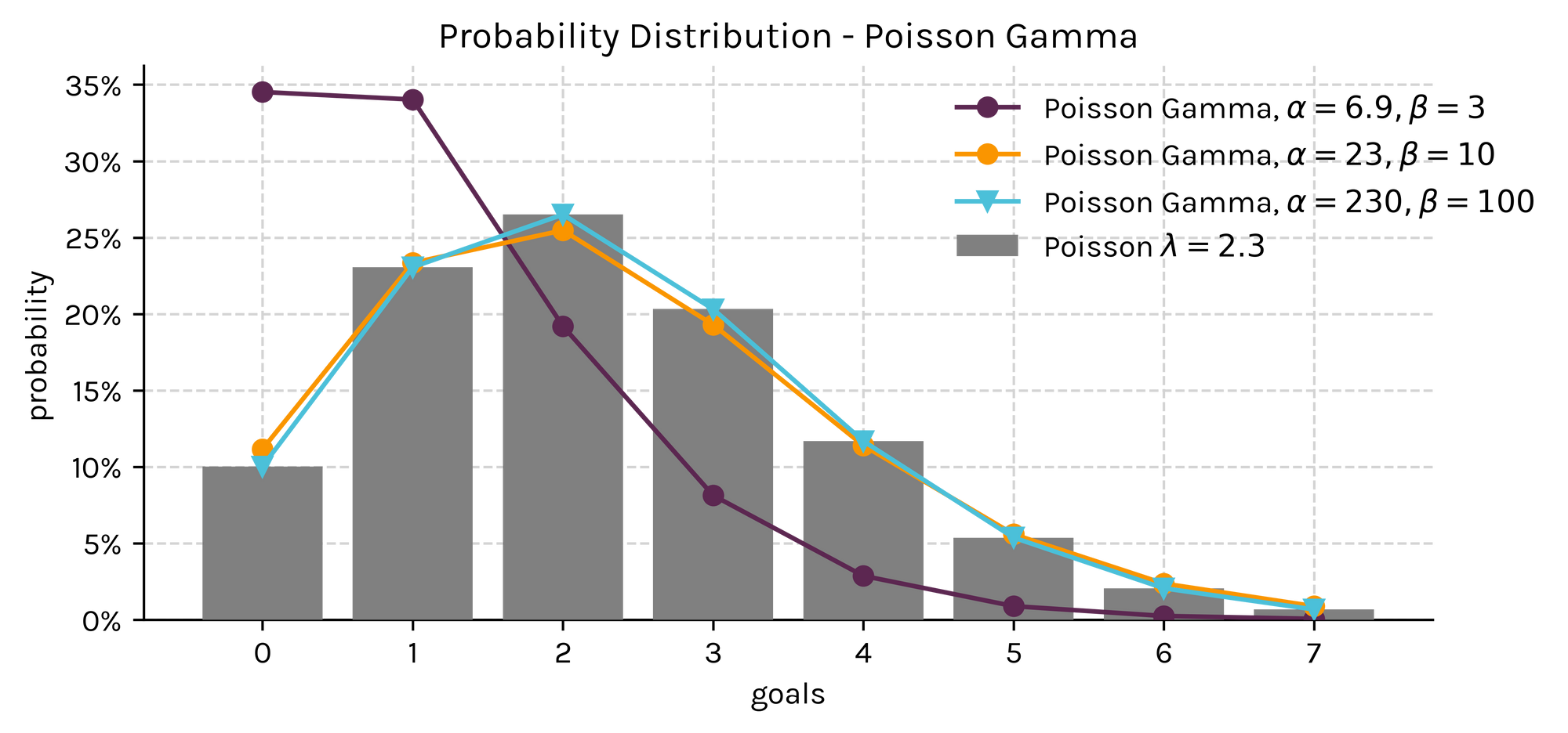
Note how the small sampled purple line assigns much higher probabilities to low scoring events given the higher presence of uncertainty on the team's goal rate; whereas, the orange and blue lines are much closer to a true Poisson distribution with a lambda equal to 2.3.
This management of uncertainty is one, if not the most important, benefit of taking a Bayesian approach.
Incorporating Data & the Posterior Distribution
Ok, now that we've covered the concept of priors, it's time to add some data to our base model.
For this, let's say we collect a sample of the random variable \(X\) (the number of goals) consisting of \(n\) matches, and for which the predicted value \(x^*\) is independent of \(x_{(n)}\) (the sample) given the goal rate (\(\lambda)\). We then have a similar expression to the one above, where \[\mathrm{Pr}(X^* | x_{(n)}) = \int_0^\infty\mathrm{Pr}(X^* | \lambda)\mathrm{Pr}(\lambda | x_{(n)})d\lambda.\]
This expression simply presents the probability of the predicted value, given the arrival of new information for \(\lambda\), i.e. the sample of matches collected. The arrival and addition of new information into our distribution is what is usually called as the posterior distribution.
To solve the integral, we can use Bayes Theorem to help us update our prior beliefs, since \[ \mathrm{Pr}(\lambda | x_{(n)}) = \frac{\mathrm{Pr}(x_{(n)} | \lambda) \mathrm{Pr}(\lambda)}{\mathrm{Pr}(x_{(n)})}, \] where \(\mathrm{Pr}(x_{(n)} | \lambda)\) is simply the maximum likelihood function of the sample.
Then, after a couple of algebraic manipulations, we get that \[\mathrm{Pr}(\lambda | x_{(n)}) \sim \mathrm{Gamma}\left(\sum_{i=0}^nx_i + \alpha, \beta + n\right),\] which is once again a Gamma function that now has a shape parameter equal to our choice of \(\alpha\) plus the observed sample of goals scored, and a rate parameter equal to our choice of \(\beta\) plus the size of the sample collected.
This result is massive, since it allows the decision maker to incorporate their beliefs naturally into the model without breaking any of the axioms of probability theory.
Finally, as we saw in the case of the prior distribution, the mix of a Gamma and Poisson distributions result in a Poisson Gamma distribution, where in this case is expressed as follows
\[ \begin{align*} \mathrm{Pr}(X^* | x_{(n)}) = \frac{\Gamma(\sum x_i + x^* + \alpha)}{\Gamma(\sum x_i + \alpha)\Gamma(x^* + 1)}p^{\sum x_i + \alpha}(1-p)^{x^*}, \end{align*} \]
where \(\alpha, \beta > 0\) are the prior parameters of the Gamma distribution and \(p = (\beta + n)(\beta+n+1)^{-1}\).
Awesome, right?
Remeber, the key thing is that we're now working with a probability distribution that mixes our prior beliefs on what might happen in the match regardless of previous scoring data, and a sample of observations.
How much weight is assigned to your hunch and how much to the data?
That's entirely up to you 😎
A Final Example
To close the article, let's retake our previous example of the match between Bayesian Wanderers and Frequentist Albion.
However, now let's assume that we collect a sample of 15 matches in which Bayesian Wanderers scored 23 goals, and that we keep our prior beliefs that the Bayesians would have scored an average of 2.3 goals per match against their opponents.
How would the final posterior distribution look like in this case?
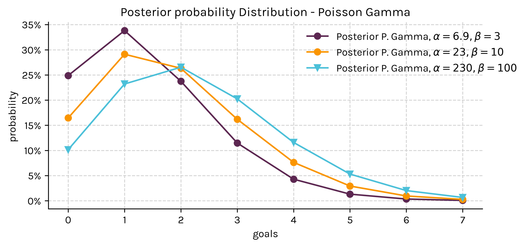
Quite different, right?
As expected, the sample has a stronger effect on the distributions with less confident priors since most of the weight is now passed to the actual data.
Closing remarks
Why is this useful?
Suppose we wish to forecast a match where the most recent or underlying data might not give us all of the information we need to accurately predict what might happen in the future. This could be anything from injuries to key players, changes in the coaching staff, or simply factors related to playing style between both teams.
By sticking to a frequentist approach we are limited to what the data tells us and we're missing the common sense factor in our prediction.
The beauty of the Bayesian approach is that we are able to add this information into the model as a true measure of uncertainty, which is dependent on our perception of the event, and all of it is done without breaking any mathematical rules.
Amazing, don't you think?
I really hope you've learned something new from this article and stay tuned for the second part of this post where we'll build a model in Python using these concepts to forecast results in the Italian Serie A.
A favour to ask.
This has been by far the hardest post I've had to write and I would love to hear your feedback on it.


