


Hey everyone!
Welcome to a new Son of a Corner tutorial.
For today's tutorial, we'll explore the basics behind a popular computational algorithm called Monte Carlo simulation and how you can apply it to football data using Python.
By the end of this tutorial, you should get a good idea of the following:
- What Monte Carlo simulation is.
- How to perform a basic Monte Carlo simulation in Python.
- How you can apply Monte Carlo simulation to football data.
What is Monte Carlo simulation?
Monte Carlo simulation is, at its core, a simple technique that uses random sampling to simulate real-world phenomena.
In essence, Monte Carlo methods are used when we are interested in a problem that could be deterministic in principle but for which it could be hard to know the exact answer. Therefore, we leverage randomness (and a computer) to estimate our answer.
Let's start with a simple example to illustrate the idea.
Imagine your friend Bob offers you to participate in a game where he throws ten dice simultaneously. If the sum of the dice is between forty and fifty, he gives you ten dollars; else, you have to pay him two dollars.
Should you play this game?
To decide whether to play, you should first figure out the probabilities of winning some money. Yes, you can compute the likelihood of winning the game by hand; however, why struggle with some pen and paper when you can use the computer to solve the problem?
Here's where Monte Carlo methods can come in useful. Let's go ahead and solve the problem using Python.
In case you didn't know, I recently launched a paid membership program through which the community can support the improvement and content available on the website. One of the perks of becoming a member is that you get early access to tutorials – so if you consistently get value out of this site, I'd appreciate it if you'd consider joining us.
Let's begin by writing a Python program that replicates our event – the throw of ten random dice.
def throw_and_sum_n_dice(n):
    '''
    This function throws n dice and sums the results
    '''
    total = 0
    for i in range(0,n):
        throw = randint(1,6)
        total += throw
    return total
Sweet, now that we have that function defined, we can write some code that calls this function a million times and then computes how often we would've won some money.
iterations = 1000000
winning_occurances = 0
for i in range(iterations):
    total = throw_and_sum_n_dice(10)
    if total >= 40 and total <= 50:
        winning_occurances += 1

print(f'We would\'ve won money {winning_occurances:,.0f} times -- a.k.a. {winning_occurances/iterations:.3%} of the time.')
>> We would've won money 202,691 times -- a.k.a. 20.269% of the time.
Interesting. It looks as though we have a 20% chance of winning ten dollars and an 80% chance of losing two bucks, which means that the game is slightly in our favor in terms of expected value.
\[\begin{align*} \text{Expected value} &= 10 \times 20\% -2 \times 80\%\\ &= 0.39 \end{align*}\](It looks like Bob doesn't know about Monte Carlo simulation 😉)
An important thing to note here is that even though we have a positive expected value, it is highly likely that if we only play once, we'll lose some money.
So let's imagine an alternative scenario where we convince Bob to let us play this game fifty times in a row, and at the end of the rounds, we distribute the payouts. How many paths would lead us to some profit?
Let's use Monte Carlo once more to get the results.
We begin by defining our function that computes the total payout after \(k\) throws.
def compute_profit_path(k, n):
    '''
    This function returns the porfit (or loss) path at the end of
    k iterations of the game, and where we throw n dice.
    '''
    total_profit = 0
    for i in range(k):
        total = throw_and_sum_n_dice(n)
        if total >= 40 and total <= 50:
            total_profit += 10
        else:
            total_profit += -2
    return total_profit
Then, we perform Monte Carlo by simulating a hundred thousand alternative paths and computing some basic descriptive statistics with the results.
iterations = 100000
total_profits = []
for i in range(iterations):
    total_profits.append(compute_profit_path(50,10))
Let's look at what could happen if we played this game.
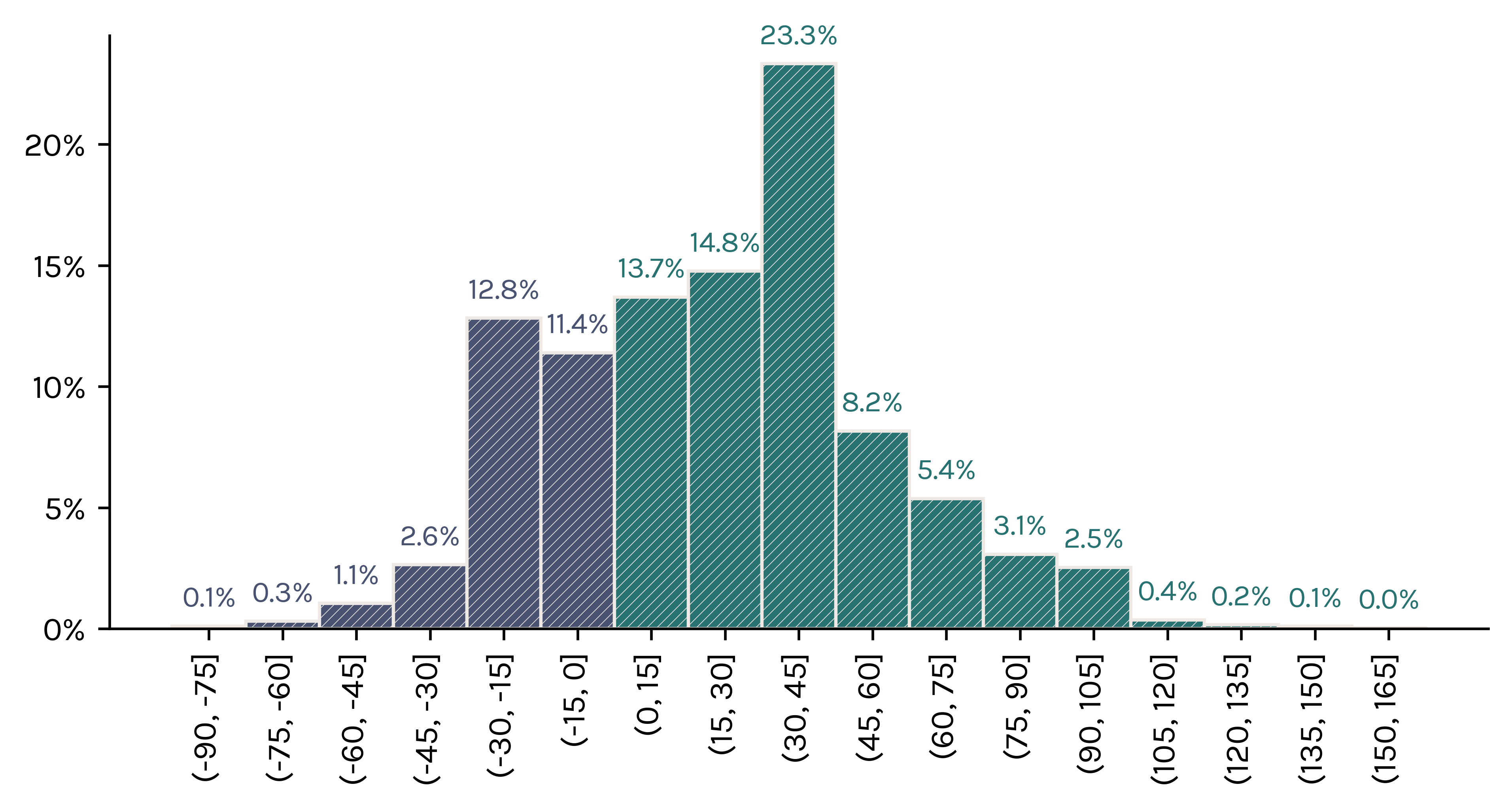
- We would win at least some money 71.7% of the time.
- Our simulation estimated that the maximum amount we could win is 152 dollars.
- Our simulation estimated that the maximum amount we could lose is 76 dollars.
- The most common outcome is that we win 20 dollars, which happens 14.8% of the time.
- We would win more than 10 dollars in 58.0% of scenarios.
- We would lose more than 10 dollars in 17.0% of scenarios.
Not bad for a day's work.
📝 Recap
A Monte Carlo simulation is a computational algorithm that leverages randomness to estimate a solution for problems of a deterministic nature or that have a probabilistic interpretation.
To perform a Monte Carlo simulation you must:
- Define the statistical properties of the inputs of your experiment. In our example of the dice, this is the probability that the faces of our ten dice will sum up to a certain number.
- Perform a large number of repetitions for your experiment – the million throws of our ten dice.
- Use the results of the repetitions to estimate the answer to the problem – in our case, whether we have a chance of winning some money from Bob.
Now that we have that covered, let's go ahead and apply these concepts to some football data.
Applying Monte Carlo Simulation to Football Data
There are countless applications to Monte Carlo simulation within the football space. In this tutorial, we'll focus on solving a simple problem in detail so that you can understand the basics and then apply these concepts to your own analysis.
The problem we'll focus on consists of estimating the probability that a certain team either wins, loses, or draws a particular match based on the quality of the chances created – the output should provide a good assessment of a team's performance, and how lucky (or not) they were to get their actual results.
Let's start by defining the problem.
First of all, let's assume that a shot's xG (expected goals) equals the probability that the shot resulted in a goal. Then, for any match, we can iterate over each shot and perform a Bernoulli trial to simulate whether the shot resulted in a goal or a miss.
For simplicity, we assume that all shots are independent of each other. This is important – and may not be entirely correct – because it allows us to sum up the outcomes of our experiment without having to worry about the correlation between the events.
By replaying this simulation multiple times, we can then use the results to estimate the probability of each outcome within the fixture.
Sound good?
Let's put it to the test with some actual data, and simulate the probabilities of each match during the group stage to see which were the most unlikely results.
Loading the data
I have supplied a dataset containing all of the shots taken in the UEFA Champions League Group stage.
df = pd.read_csv('data/ucl_shot_data.csv', index_col=0)
# -- We filter own goals since they have no xG
df = df[df['is_own_goal'] == False]
df.head()
| | shot_id | event_type | team_id | player_id | player_name | shot_x | shot_y | min | min_added | is_blocked | is_on_target | blocked_x | blocked_y | goal_crossed_y | goal_crossed_z | xG | xGOT | shot_type | situation | period | is_own_goal | on_goal_x | on_goal_y | match_id | short_name | team_name |
|---:|-----------:|:-------------|----------:|------------:|:-------------------|---------:|---------:|------:|------------:|:-------------|:---------------|------------:|------------:|-----------------:|-----------------:|----------:|---------:|:------------|:------------|:----------|:--------------|------------:|------------:|-----------:|-------------:|:-----------------|
| 0 | 2456730363 | Miss | 178475 | 450980 | Timo Werner | 98.0526 | 48.1345 | 3 | nan | False | False | nan | nan | 41.5991 | 3.13352 | 0.0951161 | nan | LeftFoot | FastBreak | FirstHalf | False | 0 | 36.5723 | 4010151 | nan | RB Leipzig |
| 1 | 2456736539 | AttemptSaved | 178475 | 704523 | Christopher Nkunku | 90.2 | 37.2025 | 12 | nan | True | True | 93 | 36.8975 | 35.4488 | 1.22 | 0.0719939 | nan | RightFoot | FromCorner | FirstHalf | False | 27.753 | 14.239 | 4010151 | nan | RB Leipzig |
| 2 | 2456736981 | AttemptSaved | 178475 | 704523 | Christopher Nkunku | 97.9561 | 36.9738 | 12 | nan | False | True | 103.293 | 35.22 | 34.9913 | 0.488 | 0.138567 | 0.091 | RightFoot | RegularPlay | FirstHalf | False | 33.1994 | 5.69561 | 4010151 | nan | RB Leipzig |
| 3 | 2456739727 | Goal | 9728 | 620543 | Maryan Shved | 75.9529 | 40.8057 | 16 | nan | False | True | nan | nan | 31.0263 | 0.160526 | 0.133662 | 0.5745 | LeftFoot | RegularPlay | FirstHalf | False | 80.4018 | 1.87356 | 4010151 | nan | Shakhtar Donetsk |
| 4 | 2456747617 | Miss | 178475 | 388523 | André Silva | 81.3587 | 37.2025 | 29 | nan | False | False | nan | nan | 24.3496 | 2.13821 | 0.0646847 | nan | RightFoot | RegularPlay | FirstHalf | False | 229.773 | 24.9558 | 4010151 | nan | RB Leipzig |Additional to the shot data, we also have a match info dataset that contains all of the information regarding the matches. This will come in useful to assess and iterate over our results.
match_data = pd.read_csv('data/match_info_data.csv', index_col=0)
match_data.head()
| | date | match_id | home_team_id | home_team_name | away_team_id | away_team_name | home_team_score | away_team_score | finished | cancelled | result | league_id | league_name |
|---:|:--------------------|-----------:|---------------:|:-----------------|---------------:|:-----------------|------------------:|------------------:|:-----------|:------------|:---------|------------:|:-----------------|
| 0 | 2022-09-07 18:45:00 | 4010118 | 8593 | Ajax | 8548 | Rangers | 4 | 0 | True | False | Home | 42 | Champions League |
| 1 | 2022-09-07 21:00:00 | 4010119 | 9875 | Napoli | 8650 | Liverpool | 4 | 1 | True | False | Home | 42 | Champions League |
| 2 | 2022-09-07 21:00:00 | 4010138 | 9906 | Atletico Madrid | 9773 | FC Porto | 2 | 1 | True | False | Home | 42 | Champions League |
| 3 | 2022-09-07 21:00:00 | 4010139 | 8342 | Club Brugge | 8178 | Leverkusen | 1 | 0 | True | False | Home | 42 | Champions League |
| 4 | 2022-09-07 21:00:00 | 4010163 | 8634 | Barcelona | 6033 | Viktoria Plzen | 5 | 1 | True | False | Home | 42 | Champions League |Simulating a match
Ok, now it's time to get down to the nitty-gritty. Writing code that simulates a single random experiment of our match.
Take a careful look at the function below, and try to make sense of what it does. However, don't worry if it's not clear, we'll explain it in just a moment.
def simulate_match_on_shots(match_id, shot_df, home_team_id, away_team_id):
    '''
    This function takes a match ID and simulates an outcome based on the shots
    taken by each team.
    '''

    shots = shot_df[shot_df['match_id'] == match_id]

    shots_home = shots[shots['team_id'] == home_team_id]
    shots_away = shots[shots['team_id'] == away_team_id]

    home_goals = 0
    # If shots == 0 then there's no sampling
    if shots_home['xG'].shape[0] > 0:
        for shot in shots_home['xG']:
            # Sample a number between 0 and 1
            prob = np.random.random()
            # If the probability sampled is less than the xG then it's a goal.
            if prob < shot:
                home_goals += 1
    away_goals = 0
    if shots_away['xG'].shape[0] > 0:
        for shot in shots_away['xG']:
            # Sample a number between 0 and 1
            prob = np.random.random()
            # If the probability sampled is less than the xG then it's a goal.
            if prob < shot:
                away_goals += 1
    return {'home_goals':home_goals, 'away_goals':away_goals}
Here's what the code does:
- We first filter our shot
DataFrameand split it into two. One for the home team, and one for the away team. - Next, we iterate over each shot taken by each side and flip a biased coin to count the occasions where the shot was randomly sampled as a goal. This is done by generating a number between 0 and 1; if the number sampled is less than the shot's xG then it's a goal, else it's a miss. Notice how the higher the xG, the higher the chance that the outcome's a goal.
- We sum up the results in each iteration and return a random scoreline.
Estimating the probabilities
Great. Now that we can generate a random scoreline, it's time to perform a Monte Carlo simulation.
To do this, we generate a large number of random scorelines and count the number of times each result (home win, draw and away win) occurred. Then, we divide that number by the total of scorelines generated.
Simple, right?
Let's write the code.
def iterate_k_simulations_on_match_id(match_id, shot_df, match_info, k=10000):
    '''
    Performs k simulations on a match, and returns the probabilites of a win, loss, draw.
    '''
    # Count the number of occurances
    home = 0
    draw = 0
    away = 0
    # Get the teams
    home_team_id = match_info[match_info['match_id'] == match_id]['home_team_id'].iloc[0]
    away_team_id = match_info[match_info['match_id'] == match_id]['away_team_id'].iloc[0]
    for i in range(k):
        simulation = simulate_match_on_shots(match_id, shot_df, home_team_id, away_team_id)
        if simulation['home_goals'] > simulation['away_goals']:
            home += 1
        elif simulation['home_goals'] < simulation['away_goals']:
            away += 1
        else:
            draw += 1
    home_prob = home/k
    draw_prob = draw/k
    away_prob = away/k
    return {'home_prob': home_prob, 'away_prob': away_prob, 'draw_prob': draw_prob, 'match_id': match_id}
For example, let's perform 10,000 simulations over the Ajax vs. Rangers match (match_id = 4010118 ).
iterate_k_simulations_on_match_id(4010118, df, match_data)>> {'home_prob': 0.8827,
'away_prob': 0.0114,
'draw_prob': 0.1059,
'match_id': 4010118}Cool! It looks as if that game had been replayed 10,000 times Ajax would've won 88% of the time – they actually won that game 4 - 0.
Wrapping things up
Now that we have a function that replays a match k times and returns us the estimated probabilities, let's then simulate all the matches in the group stage to find the most unlikely results.
(this can take a few minutes, so it's a good excuse to go get a cup of coffee ☕️)
match_probs = []
for index, match in enumerate(match_data['match_id']):
    outcome_probs = iterate_k_simulations_on_match_id(match, df, match_data)
    match_probs.append(outcome_probs)
    if index % 10 == 0:
        print(f'{index/match_data.shape[0]:.1%} done.')
When that's done, we convert our results into a DataFrame and merge it with our match_data dataset.
match_probs_df = pd.DataFrame(match_probs)
final_df = pd.merge(match_data, match_probs_df, on='match_id')
final_df.head()
The output should look something like this...
|    | date                |   match_id |   home_team_id | home_team_name   |   away_team_id | away_team_name   |   home_team_score |   away_team_score | finished   | cancelled   | result   |   league_id | league_name      |   home_prob |   draw_prob |   away_prob |
|---:|:--------------------|-----------:|---------------:|:-----------------|---------------:|:-----------------|------------------:|------------------:|:-----------|:------------|:---------|------------:|:-----------------|------------:|------------:|------------:|
|  0 | 2022-09-07 18:45:00 |    4010118 |           8593 | Ajax             |           8548 | Rangers          |                 4 |                 0 | True       | False       | Home     |          42 | Champions League |      0.8818 |      0.1065 |      0.0117 |
|  1 | 2022-09-07 21:00:00 |    4010119 |           9875 | Napoli           |           8650 | Liverpool        |                 4 |                 1 | True       | False       | Home     |          42 | Champions League |      0.9472 |      0.0377 |      0.0151 |
|  2 | 2022-09-07 21:00:00 |    4010138 |           9906 | Atletico Madrid  |           9773 | FC Porto         |                 2 |                 1 | True       | False       | Home     |          42 | Champions League |      0.0868 |      0.1972 |      0.716  |
|  3 | 2022-09-07 21:00:00 |    4010139 |           8342 | Club Brugge      |           8178 | Leverkusen       |                 1 |                 0 | True       | False       | Home     |          42 | Champions League |      0.1627 |      0.3324 |      0.5049 |
|  4 | 2022-09-07 21:00:00 |    4010163 |           8634 | Barcelona        |           6033 | Viktoria Plzen   |                 5 |                 1 | True       | False       | Home     |          42 | Champions League |      0.7315 |      0.1768 |      0.0917 |
Assessing the results
To evaluate each team's performance, we'll perform a statistical test to see which were the most unlikely results. For this, we'll be using the Brier Score function which is designed to compute the accuracy of probabilistic predictions. Even though we weren't forecasting anything here, it will show which results were the most unlikely.
The BS definition is:
\[\text{BS} = (P_h - o_h)^2 + (P_d - o_d)^2 + (P_a - o_a)^2\]
where: \(P\) denotes the probability of a home win, draw, and away win, respectively; and \(o = 1\) in case the outcome occurred and \(0\), otherwise.
Here's the code to achieve that:
final_df['home_result'] = [1 if x == 'Home' else 0 for x in final_df['result']]
final_df['draw_result'] = [1 if x == 'Draw' else 0 for x in final_df['result']]
final_df['away_result'] = [1 if x == 'Away' else 0 for x in final_df['result']]
final_df['brier_score'] = (
(final_df['home_prob'] - final_df['home_result'])**2 +
(final_df['draw_prob'] - final_df['draw_result'])**2 +
(final_df['away_prob'] - final_df['away_result'])**2
)Finally, we take a look at the twenty most unlikely results
result_df = final_df.drop(['date','match_id','home_team_id','away_team_id','cancelled','finished','league_id','league_name','home_result','away_result','draw_result'], axis=1)
result_df.sort_values(by='brier_score',ascending=False).head(20)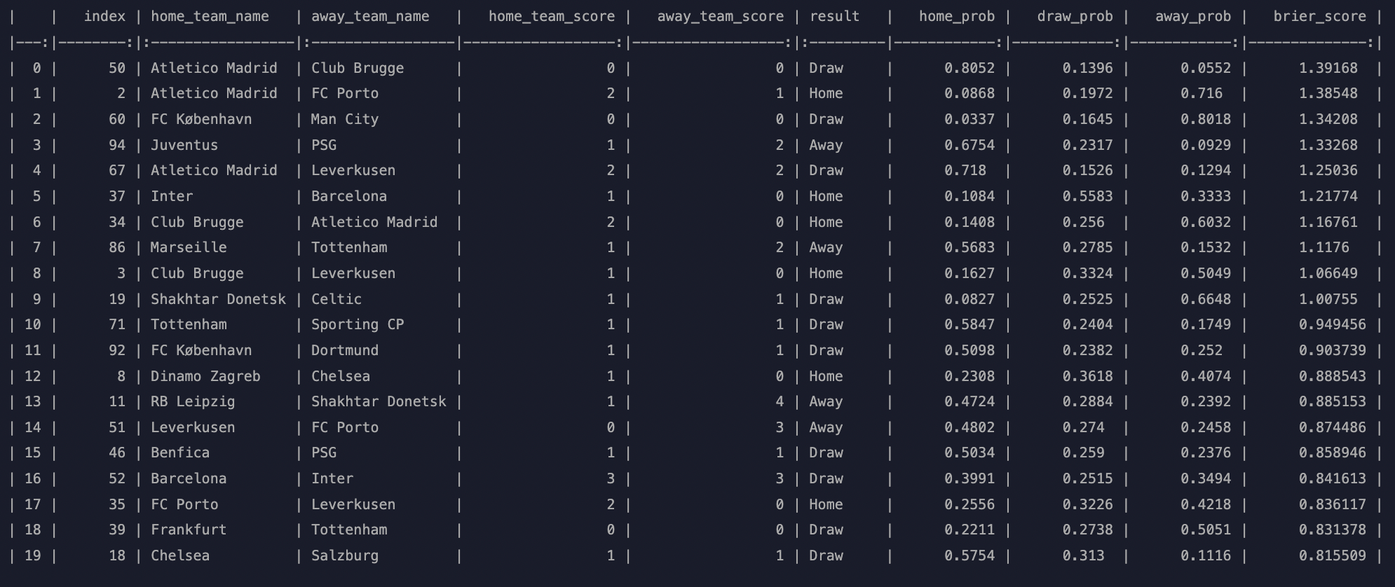
WOW! Four of Atlético Madrid's games rank in the top seven most unlikely games – although with some in their favor.
So there you have it, that's one example of how you can apply Monte Carlo simulation to football data. Hope you learned something new from this tutorial and I'll catch you later 😎
📝 Optional Excercise
If you want to put your skills to the test I suggest you extend the above example and simulate each team's chances of passing to the round of sixteen.
Can you figure out how to do it?


